PivotTables – using the Summary functions

Today, let us learn a bit about PivotTables and the convenient assistance they offer us in many ways. This tip is based on a special request from one of my friends P Sreenath, who wanted me to write a few things on Pivots.

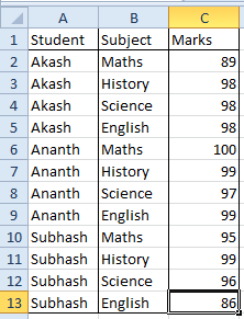
Let us take an example to understand the summary functions better. Consider the following table of student and subject-wise academic performance (data of marks scored):

Now, the school management wants to do a summary analysis by subject and find out the maximum marks scored, the minimum marks scored and the average marks scored, so that they can evaluate the respective subject teachers. 

Since the data is available by student, if we need to get the summary level data by subjects, we must sort the data by subjects and then use the MAX, MIN and AVERAGE worksheet functions on each data range to get the values of maximum, minimum and average scores respectively - see the restructured sample below.

However, there is an easier option available and would be a boon especially when you have a huge number of records to work on. You can forget the manual methods of sorting and applying formula to each selected range of subjects and three different forumulas for each one – in this current example, 4 subjects x 3 functions each = altogether 12 formulas to be setup manually. 

Take recourse to the PivotTables, and let us find an easy solution. Just follow these steps:

Step 1: Select the data range, and click on the PivotTable button on the Insert menu of the Ribbon.

Step 2: Choose your option of New worksheet or existing place in the current worksheet, to get the PivotTable skeleton structure.

Step 3: Drag the Subject field to the Row Labels zone, and drag the Marks field thrice to the Values zone – as shown below:

Step 4: Now click on the first Marks field (“Sum of Marks” in the values zone) and select Value Field settings. In the dialog box, just select the function MAX (instead of the default sum) and click ok.

Step 5: Repeat the process on “Sum of Marks2” – making it MIN and “Sum of Marks3” – making it AVERAGE. Your work is done in a jiffy now. See the summary results below.

Note: 

When you do the average, you will note that there are too many decimals that appear. If you want your worksheet to look clean and without decimals, you can use the value field settings again on that field, select the Number Format button which will bring up the Cell properties dialog box. You can set the field to Number type with zero decimal places there and click OK. Note that the number formatting would be retained on the PivotTable only when you set it through the Value Settings dialog box. If you use the comma button or $ button on the Ribbon to format the cells, the formatting would be lost the next time the Pivot is refreshed. 

The example file is available on Skydrive for you to take a quick online view  - http://sdrv.ms/SsLOOa

Hope you will find this tip useful and handy. I will try to share few more interesting tips on PivotTables in the coming days as well. Would be glad to have your comments on this, and help your friends also to learn a trick or two – share the blog details with them!

My upcoming book on Excel contains many more such tricks and practical insights into getting Excel work for you. Please take a moment to visit my earlier post to understand details about my new book, and make use of the special offer available now to order it at a discount.